Using the Fixed Variance process
The FixedVariance volatility process can be used to implement zig-zag model estimation where two steps are repeated until convergence. This can be used to estimate models which may not be easy to estimate as a single process due to numerical issues or a high-dimensional parameter space.
This setup code is required to run in an IPython notebook
[1]:
import matplotlib.pyplot as plt
import seaborn

seaborn.set_style("darkgrid")
plt.rc("figure", figsize=(16, 6))
plt.rc("savefig", dpi=90)
plt.rc("font", family="sans-serif")
plt.rc("font", size=14)
Setup
Imports used in this example.
[2]:
import numpy as np
Data
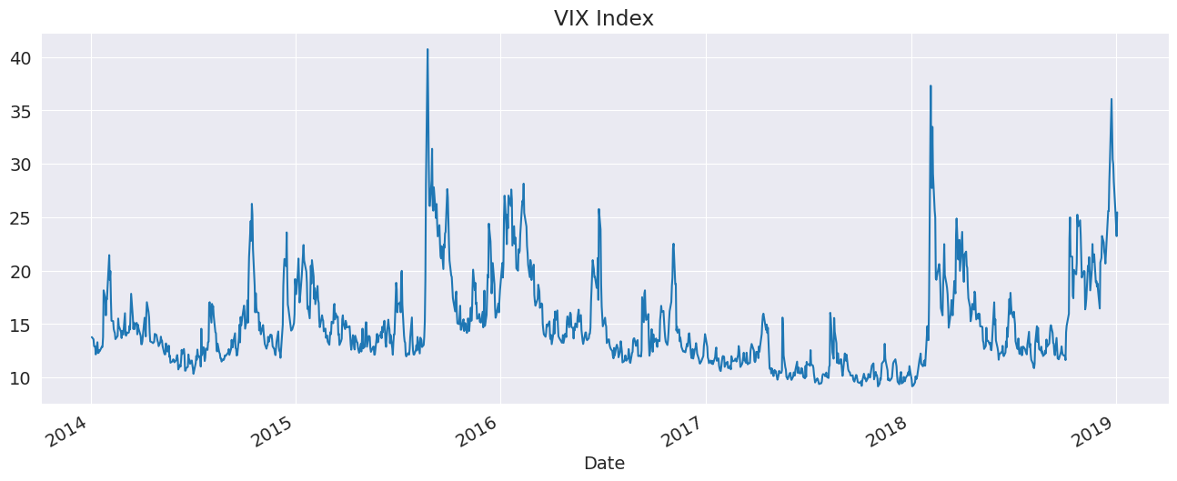
The VIX index will be used to illustrate the use of the FixedVariance process. The data is from FRED and is provided by the arch package.
[3]:
import arch.data.vix

vix_data = arch.data.vix.load()
vix = vix_data.vix.dropna()
vix.name = "VIX Index"
ax = vix.plot(title="VIX Index")
Initial Mean Model Estimation
The first step is to estimate the mean to filter the residuals using a constant variance.
[4]:
from arch.univariate.mean import HARX, ZeroMean
from arch.univariate.volatility import GARCH, FixedVariance

mod = HARX(vix, lags=[1, 5, 22])
res = mod.fit()
print(res.summary())
                    HAR - Constant Variance Model Results
==============================================================================
Dep. Variable:              VIX Index   R-squared:                       0.876
Mean Model:                       HAR   Adj. R-squared:                  0.876
Vol Model:          Constant Variance   Log-Likelihood:               -2267.95
Distribution:                  Normal   AIC:                           4545.90
Method:            Maximum Likelihood   BIC:                           4571.50
                                        No. Observations:                 1237
Date:                Tue, Nov 05 2024   Df Residuals:                     1233
Time:                        09:03:40   Df Model:                            4
                                   Mean Model
================================================================================
                      coef    std err          t      P>|t|     95.0% Conf. Int.
--------------------------------------------------------------------------------
Const               0.6335      0.189      3.359  7.831e-04    [  0.264,  1.003]
VIX Index[0:1]      0.9287  6.589e-02     14.095  4.056e-45    [  0.800,  1.058]
VIX Index[0:5]     -0.0318  6.449e-02     -0.492      0.622  [ -0.158,9.463e-02]
VIX Index[0:22]     0.0612  3.180e-02      1.926  5.409e-02 [-1.076e-03,  0.124]
                            Volatility Model
========================================================================
                 coef    std err          t      P>|t|  95.0% Conf. Int.
------------------------------------------------------------------------
sigma2         2.2910      0.396      5.782  7.361e-09 [  1.514,  3.068]
========================================================================

Covariance estimator: White's Heteroskedasticity Consistent Estimator
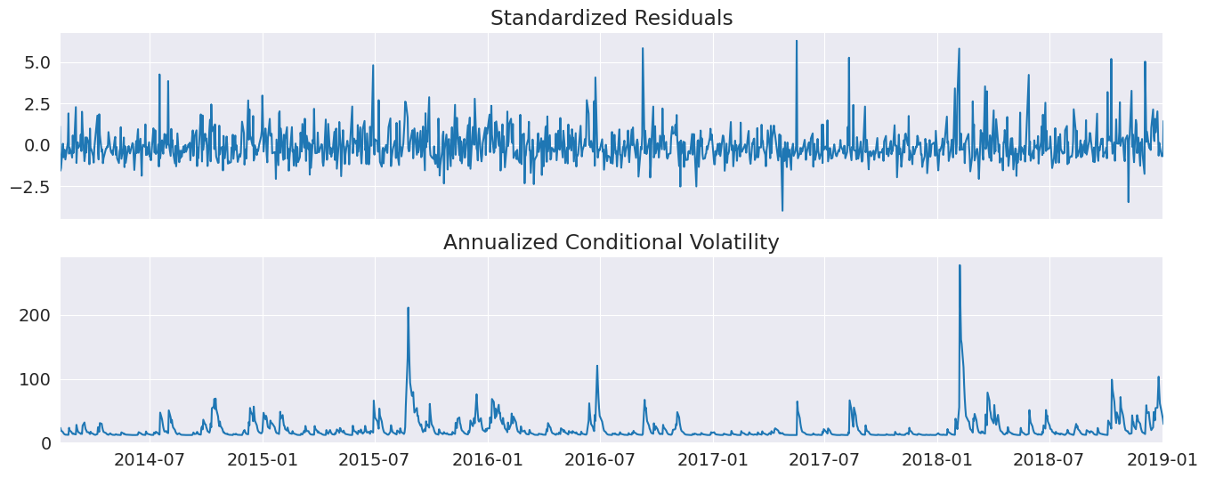
Initial Volatility Model Estimation
Using the previously estimated residuals, a volatility model can be estimated using a ZeroMean. In this example, a GJR-GARCH process is used for the variance.
[5]:
vol_mod = ZeroMean(res.resid.dropna(), volatility=GARCH(p=1, o=1, q=1))
vol_res = vol_mod.fit(disp="off")
print(vol_res.summary())
                     Zero Mean - GJR-GARCH Model Results
==============================================================================
Dep. Variable:                  resid   R-squared:                       0.000
Mean Model:                 Zero Mean   Adj. R-squared:                  0.001
Vol Model:                  GJR-GARCH   Log-Likelihood:               -1936.93
Distribution:                  Normal   AIC:                           3881.86
Method:            Maximum Likelihood   BIC:                           3902.35
                                        No. Observations:                 1237
Date:                Tue, Nov 05 2024   Df Residuals:                     1237
Time:                        09:03:40   Df Model:                            0
                              Volatility Model
===========================================================================
                 coef    std err          t      P>|t|     95.0% Conf. Int.
---------------------------------------------------------------------------
omega          0.2355  9.134e-02      2.578  9.932e-03  [5.647e-02,  0.415]
alpha[1]       0.7217      0.374      1.931  5.353e-02 [-1.098e-02,  1.454]
gamma[1]      -0.7217      0.252     -2.859  4.255e-03    [ -1.217, -0.227]
beta[1]        0.5789      0.184      3.140  1.692e-03    [  0.218,  0.940]
===========================================================================

Covariance estimator: robust
[6]:
ax = vol_res.plot("D")
Re-estimating the mean with a FixedVariance
The FixedVariance requires that the variance is provided when initializing the object. The variance provided should have the same shape as the original data. Since the variance estimated from the GJR-GARCH model is missing the first 22 observations due to the HAR lags, we simply fill these with 1. These values will not be used to estimate the model, and so the value is not important.
The summary shows that there is a single parameter, scale, which is close to 1. The mean parameters have changed which reflects the GLS-like weighting that this re-estimation imposes.
[7]:
variance = np.empty_like(vix)
variance.fill(1.0)
variance[22:] = vol_res.conditional_volatility**2.0
fv = FixedVariance(variance)
mod = HARX(vix, lags=[1, 5, 22], volatility=fv)
res = mod.fit()
print(res.summary())
Iteration:      1,   Func. Count:      7,   Neg. LLF: 255807077112.90338
Iteration:      2,   Func. Count:     19,   Neg. LLF: 930291.8228765851
Iteration:      3,   Func. Count:     28,   Neg. LLF: 3486.703789639719
Iteration:      4,   Func. Count:     36,   Neg. LLF: 2885.6851427633
Iteration:      5,   Func. Count:     44,   Neg. LLF: 65536161.73048766
Iteration:      6,   Func. Count:     53,   Neg. LLF: 1935.9527542814274
Iteration:      7,   Func. Count:     59,   Neg. LLF: 1935.9470521012404
Iteration:      8,   Func. Count:     65,   Neg. LLF: 1935.947051490633
Optimization terminated successfully    (Exit mode 0)
            Current function value: 1935.947051490633
            Iterations: 8
            Function evaluations: 65
            Gradient evaluations: 8
                      HAR - Fixed Variance Model Results
==============================================================================
Dep. Variable:              VIX Index   R-squared:                       0.876
Mean Model:                       HAR   Adj. R-squared:                  0.876
Vol Model:             Fixed Variance   Log-Likelihood:               -1935.95
Distribution:                  Normal   AIC:                           3881.89
Method:            Maximum Likelihood   BIC:                           3907.50
                                        No. Observations:                 1237
Date:                Tue, Nov 05 2024   Df Residuals:                     1233
Time:                        09:03:41   Df Model:                            4
                                    Mean Model
==================================================================================
                      coef    std err          t      P>|t|       95.0% Conf. Int.
----------------------------------------------------------------------------------
Const               0.5584      0.153      3.661  2.507e-04      [  0.260,  0.857]
VIX Index[0:1]      0.9376  3.625e-02     25.866 1.607e-147      [  0.867,  1.009]
VIX Index[0:5]     -0.0249  3.782e-02     -0.657      0.511 [-9.899e-02,4.926e-02]
VIX Index[0:22]     0.0493  2.102e-02      2.344  1.909e-02  [8.064e-03,9.044e-02]
                            Volatility Model
========================================================================
                 coef    std err          t      P>|t|  95.0% Conf. Int.
------------------------------------------------------------------------
scale          0.9986  8.081e-02     12.358  4.420e-35 [  0.840,  1.157]
========================================================================

Covariance estimator: robust
Zig-Zag estimation
A small repetitions of the previous two steps can be used to implement a so-called zig-zag estimation strategy.
[8]:
for i in range(5):
    print(i)
    vol_mod = ZeroMean(res.resid.dropna(), volatility=GARCH(p=1, o=1, q=1))
    vol_res = vol_mod.fit(disp="off")
    variance[22:] = vol_res.conditional_volatility**2.0
    fv = FixedVariance(variance, unit_scale=True)
    mod = HARX(vix, lags=[1, 5, 22], volatility=fv)
    res = mod.fit(disp="off")
print(res.summary())
0
1
2
3
4
                    HAR - Fixed Variance (Unit Scale) Model Results
=======================================================================================
Dep. Variable:                       VIX Index   R-squared:                       0.876
Mean Model:                                HAR   Adj. R-squared:                  0.876
Vol Model:         Fixed Variance (Unit Scale)   Log-Likelihood:               -1935.74
Distribution:                           Normal   AIC:                           3879.48
Method:                     Maximum Likelihood   BIC:                           3899.96
                                                 No. Observations:                 1237
Date:                         Tue, Nov 05 2024   Df Residuals:                     1233
Time:                                 09:03:41   Df Model:                            4
                                    Mean Model
=================================================================================
                      coef    std err          t      P>|t|      95.0% Conf. Int.
---------------------------------------------------------------------------------
Const               0.5602      0.152      3.681  2.324e-04     [  0.262,  0.858]
VIX Index[0:1]      0.9381  3.616e-02     25.939 2.389e-148     [  0.867,  1.009]
VIX Index[0:5]     -0.0262  3.774e-02     -0.693      0.488   [ -0.100,4.781e-02]
VIX Index[0:22]     0.0499  2.099e-02      2.380  1.733e-02 [8.810e-03,9.109e-02]
=================================================================================

Covariance estimator: robust
Direct Estimation
This model can be directly estimated. The results are provided for comparison to the previous FixedVariance estimates of the mean parameters.
[9]:
mod = HARX(vix, lags=[1, 5, 22], volatility=GARCH(1, 1, 1))
res = mod.fit(disp="off")
print(res.summary())
                        HAR - GJR-GARCH Model Results
==============================================================================
Dep. Variable:              VIX Index   R-squared:                       0.876
Mean Model:                       HAR   Adj. R-squared:                  0.875
Vol Model:                  GJR-GARCH   Log-Likelihood:               -1932.61
Distribution:                  Normal   AIC:                           3881.23
Method:            Maximum Likelihood   BIC:                           3922.19
                                        No. Observations:                 1237
Date:                Tue, Nov 05 2024   Df Residuals:                     1233
Time:                        09:03:41   Df Model:                            4
                                   Mean Model
================================================================================
                      coef    std err          t      P>|t|     95.0% Conf. Int.
--------------------------------------------------------------------------------
Const               0.7796      1.190      0.655      0.513    [ -1.554,  3.113]
VIX Index[0:1]      0.9180      0.291      3.156  1.597e-03    [  0.348,  1.488]
VIX Index[0:5]     -0.0393      0.296     -0.133      0.894    [ -0.620,  0.541]
VIX Index[0:22]     0.0632  6.353e-02      0.994      0.320 [-6.136e-02,  0.188]
                            Volatility Model
========================================================================
                 coef    std err          t      P>|t|  95.0% Conf. Int.
------------------------------------------------------------------------
omega          0.2357      0.250      0.944      0.345 [ -0.254,  0.725]
alpha[1]       0.7091      1.069      0.664      0.507 [ -1.386,  2.804]
gamma[1]      -0.7091      0.519     -1.367      0.172 [ -1.726,  0.308]
beta[1]        0.5579      0.855      0.653      0.514 [ -1.117,  2.233]
========================================================================

Covariance estimator: robust