Forecasting with Exogenous Regressors¶

This notebook provides examples of the accepted data structures for passing the expected value of exogenous variables when these are included in the mean. For example, consider an AR(1) with 2 exogenous variables. The mean dynamics are

The \(h\)-step forecast, \(E_{T}[Y_{t+h}]\), depends on the conditional expectation of \(X_{0,T+h}\) and \(X_{1,T+h}\),

where \(E_{T}[Y_{T+h-1}]\) has been recursively computed.

In order to construct forecasts up to some horizon \(h\), it is necessary to pass \(2\times h\) values (\(h\) for each series). If using the features of forecast that allow many forecast to be specified, it necessary to supply \(n \times 2 \times h\) values.

There are two general purpose data structures that can be used for any number of exogenous variables and any number steps ahead:

• dict - The values can be pass using a dict where the keys are the variable names and the values are 2-dimensional arrays. This is the most natural generalization of a pandas DataFrame to 3-dimensions.

• array - The vales can alternatively be passed as a 3-d NumPy array where dimension 0 tracks the regressor index, dimension 1 is the time period and dimension 2 is the horizon.

When a model contains a single exogenous regressor it is possible to use a 2-d array or DataFrame where dim0 tracks the time period where the forecast is generated and dimension 1 tracks the horizon.

In the special case where a model contains a single regressor and the horizon is 1, then a 1-d array of pandas Series can be used.

[1]:

# initial setup
%matplotlib inline

import matplotlib.pyplot as plt
import numpy as np
import pandas as pd
import seaborn
from arch.__future__ import reindexing

seaborn.set_style("darkgrid")
plt.rc("figure", figsize=(16, 6))
plt.rc("savefig", dpi=90)
plt.rc("font", family="sans-serif")
plt.rc("font", size=14)

Simulating data¶

Two \(X\) variables are simulated and are assumed to follow independent AR(1) processes. The data is then assumed to follow an ARX(1) with 2 exogenous regressors and GARCH(1,1) errors.

[2]:

from arch.univariate import ARX, GARCH, ZeroMean, arch_model

burn = 250

x_mod = ARX(None, lags=1)
x0 = x_mod.simulate([1, 0.8, 1], nobs=1000 + burn).data
x1 = x_mod.simulate([2.5, 0.5, 1], nobs=1000 + burn).data

resid_mod = ZeroMean(volatility=GARCH())
resids = resid_mod.simulate([0.1, 0.1, 0.8], nobs=1000 + burn).data

phi1 = 0.7
phi0 = 3
y = 10 + resids.copy()
for i in range(1, y.shape[0]):
    y[i] = phi0 + phi1 * y[i - 1] + 2 * x0[i] - 2 * x1[i] + resids[i]

x0 = x0.iloc[-1000:]
x1 = x1.iloc[-1000:]
y = y.iloc[-1000:]
y.index = x0.index = x1.index = np.arange(1000)

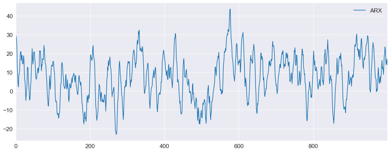
Plotting the data¶

[3]:

ax = pd.DataFrame({"ARX": y}).plot(legend=False)
ax.legend(frameon=False)
_ = ax.set_xlim(0, 999)

Forecasting the X values¶

The forecasts of \(Y\) depend on forecasts of \(X_0\) and \(X_1\). Both of these follow simple AR(1), and so we can construct the forecasts for all time horizons. Note that the value in position [i,j] is the time-i forecast for horizon j+1.

[4]:

x0_oos = np.empty((1000, 10))
x1_oos = np.empty((1000, 10))
for i in range(10):
    if i == 0:
        last = x0
    else:
        last = x0_oos[:, i - 1]
    x0_oos[:, i] = 1 + 0.8 * last
    if i == 0:
        last = x1
    else:
        last = x1_oos[:, i - 1]
    x1_oos[:, i] = 2.5 + 0.5 * last

x1_oos[-1]

[4]:

array([5.32610653, 5.16305327, 5.08152663, 5.04076332, 5.02038166,
       5.01019083, 5.00509541, 5.00254771, 5.00127385, 5.00063693])

Fitting the model¶

Next, the most is fit. The parameters are accurately estimated.

[5]:

exog = pd.DataFrame({"x0": x0, "x1": x1})
mod = arch_model(y, x=exog, mean="ARX", lags=1)
res = mod.fit(disp="off")
print(res.summary())

                          AR-X - GARCH Model Results
==============================================================================
Dep. Variable:                   data   R-squared:                       0.993
Mean Model:                      AR-X   Adj. R-squared:                  0.993
Vol Model:                      GARCH   Log-Likelihood:               -1302.15
Distribution:                  Normal   AIC:                           2618.31
Method:            Maximum Likelihood   BIC:                           2652.65
                                        No. Observations:                  999
Date:                Mon, May 17 2021   Df Residuals:                      995
Time:                        16:04:11   Df Model:                            4
                               Mean Model
========================================================================
                 coef    std err          t      P>|t|  95.0% Conf. Int.
------------------------------------------------------------------------
Const          2.9480      0.149     19.818  2.088e-87 [  2.656,  3.240]
data[1]        0.6971  3.421e-03    203.759      0.000 [  0.690,  0.704]
x0             2.0186  2.063e-02     97.827      0.000 [  1.978,  2.059]
x1            -2.0115  2.483e-02    -81.001      0.000 [ -2.060, -1.963]
                              Volatility Model
===========================================================================
                 coef    std err          t      P>|t|     95.0% Conf. Int.
---------------------------------------------------------------------------
omega          0.1144  5.879e-02      1.946  5.162e-02 [-8.041e-04,  0.230]
alpha[1]       0.0633  2.982e-02      2.123  3.374e-02  [4.866e-03,  0.122]
beta[1]        0.7940  9.035e-02      8.788  1.522e-18    [  0.617,  0.971]
===========================================================================

Covariance estimator: robust

Using a dict¶

The first approach uses a dict to pass the two variables. The key consideration here is the the keys of the dictionary must exactly match the variable names (x0 and x1 here). The dictionary here contains only the final row of the forecast values since forecast will only make forecasts beginning from the final in-sample observation by default.

Using DataFrame¶

While these examples make use of NumPy arrays, these can be DataFrames. This allows the index to be used to track the forecast origination point, which can be a helpful device.

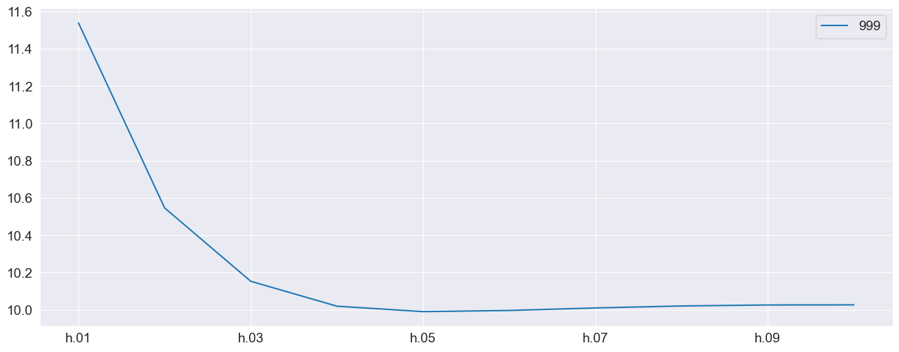
[6]:

exog_fcast = {"x0": x0_oos[-1:], "x1": x1_oos[-1:]}
forecasts = res.forecast(horizon=10, x=exog_fcast)
forecasts.mean.T.plot()

[6]:

<AxesSubplot:>

Using an array¶

An array can alternatively be used. This frees the restriction on matching the variable names although the order must match instead. The forecast values are 2 (variables) by 1 (forecast) by 10 (horizon).

[7]:

exog_fcast = np.array([x0_oos[-1:], x1_oos[-1:]])
print(f"The shape is {exog_fcast.shape}")
array_forecasts = res.forecast(horizon=10, x=exog_fcast)
print(array_forecasts.mean - forecasts.mean)

The shape is (2, 1, 10)
     h.01  h.02  h.03  h.04  h.05  h.06  h.07  h.08  h.09  h.10
999   0.0   0.0   0.0   0.0   0.0   0.0   0.0   0.0   0.0   0.0

Producing multiple forecasts¶

forecast can produce multiple forecasts using the same fit model. Here the model is fit to the first 500 observations and then forecasting for the remaining values are produced. It must be the case that the x values passed for forecast have the same number of rows as the table of forecasts produced.

[8]:

res = mod.fit(disp="off", last_obs=500)
exog_fcast = {"x0": x0_oos[-500:], "x1": x1_oos[-500:]}
multi_forecasts = res.forecast(start=500, horizon=10, x=exog_fcast)
multi_forecasts.mean.tail(10)

[8]:

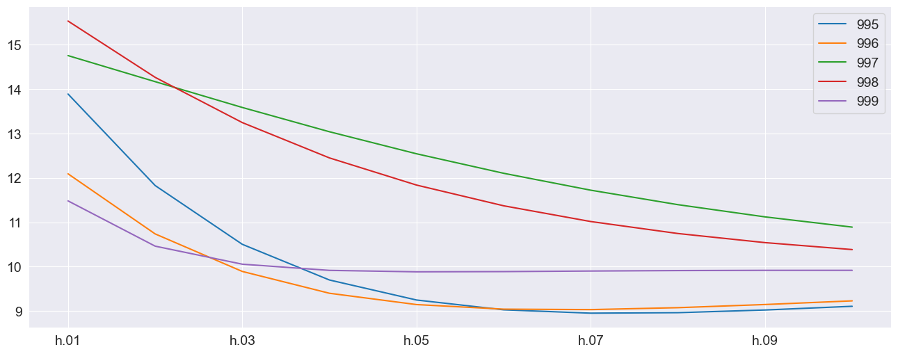
The plot of the final 5 forecast paths shows the the mean reversion of the process.

[9]:

_ = multi_forecasts.mean.tail().T.plot()

The previous example made use of dictionaries where each of the values was a 500 (number of forecasts) by 10 (horizon) array. The alternative format can be used where x is a 3-d array with shape 2 (variables) by 500 (forecasts) by 10 (horizon).

[10]:

exog_fcast = np.array([x0_oos[-500:], x1_oos[-500:]])
print(exog_fcast.shape)
array_multi_forecasts = res.forecast(start=500, horizon=10, x=exog_fcast)
np.max(np.abs(array_multi_forecasts.mean - multi_forecasts.mean))

(2, 500, 10)

[10]:

h.01    0.0
h.02    0.0
h.03    0.0
h.04    0.0
h.05    0.0
h.06    0.0
h.07    0.0
h.08    0.0
h.09    0.0
h.10    0.0
dtype: float64

x input array sizes¶

While the natural shape of the x data is the number of forecasts, it is also possible to pass an x that has the same shape as the y used to construct the model. The may simplify tracking the origin points of the forecast. Values are are not needed are ignored. In this example, the out-of-sample values are 2 by 1000 (original number of observations) by 10. Only the final 500 are used.

[11]:

exog_fcast = np.array([x0_oos, x1_oos])
print(exog_fcast.shape)
array_multi_forecasts = res.forecast(start=500, horizon=10, x=exog_fcast)
np.max(np.abs(array_multi_forecasts.mean - multi_forecasts.mean))

(2, 1000, 10)

[11]:

h.01    0.0
h.02    0.0
h.03    0.0
h.04    0.0
h.05    0.0
h.06    0.0
h.07    0.0
h.08    0.0
h.09    0.0
h.10    0.0
dtype: float64

Special Cases with a single x variable¶

When a model consists of a single exogenous regressor, then x can be a 1-d or 2-d array (or Series or DataFrame).

[12]:

mod = arch_model(y, x=exog.iloc[:, :1], mean="ARX", lags=1)
res = mod.fit(disp="off")
print(res.summary())

                          AR-X - GARCH Model Results
==============================================================================
Dep. Variable:                   data   R-squared:                       0.949
Mean Model:                      AR-X   Adj. R-squared:                  0.949
Vol Model:                      GARCH   Log-Likelihood:               -2310.31
Distribution:                  Normal   AIC:                           4632.63
Method:            Maximum Likelihood   BIC:                           4662.07
                                        No. Observations:                  999
Date:                Mon, May 17 2021   Df Residuals:                      996
Time:                        16:04:11   Df Model:                            3
                               Mean Model
========================================================================
                 coef    std err          t      P>|t|  95.0% Conf. Int.
------------------------------------------------------------------------
Const         -6.3468      0.283    -22.464 9.346e-112 [ -6.901, -5.793]
data[1]        0.7555  9.631e-03     78.446      0.000 [  0.737,  0.774]
x0             1.7840  6.195e-02     28.799 2.192e-182 [  1.663,  1.905]
                             Volatility Model
==========================================================================
                 coef    std err          t      P>|t|    95.0% Conf. Int.
--------------------------------------------------------------------------
omega          3.0493      0.753      4.052  5.085e-05   [  1.574,  4.524]
alpha[1]       0.1626  3.741e-02      4.346  1.385e-05 [8.926e-02,  0.236]
beta[1]        0.3401      0.129      2.631  8.523e-03 [8.670e-02,  0.593]
==========================================================================

Covariance estimator: robust

These two examples show that both formats can be used.

[13]:

forecast_1d = res.forecast(horizon=10, x=x0_oos[-1])
forecast_2d = res.forecast(horizon=10, x=x0_oos[-1:])
print(forecast_1d.mean - forecast_2d.mean)

## Simulation-forecasting

mod = arch_model(y, x=exog, mean="ARX", lags=1, power=1.0)
res = mod.fit(disp="off")

     h.01  h.02  h.03  h.04  h.05  h.06  h.07  h.08  h.09  h.10
999   0.0   0.0   0.0   0.0   0.0   0.0   0.0   0.0   0.0   0.0

Simulation¶

forecast supports simulating paths. When forecasting a model with exogenous variables, the same value is used to in all mean paths. If you wish to also simulate the paths of the x variables, these need to generated and then passed inside a loop.

Static out-of-sample x¶

This first example shows that variance of the paths when the same x values are used in the forecast. There is a sense the out-of-sample x are treated as deterministic.

[14]:

x = {"x0": x0_oos[-1], "x1": x1_oos[-1]}
sim_fixedx = res.forecast(horizon=10, x=x, method="simulation", simulations=100)
sim_fixedx.simulations.values.std(1)

[14]:

array([[0.94510757, 0.97700028, 1.13035701, 1.10824845, 1.26825095,
        1.26590793, 1.23342443, 1.18098812, 1.28265677, 1.2315994 ]])

Simulating the out-of-sample x¶

This example simulates distinct paths for the two exogenous variables and then simulates a single path. This is then repeated 100 times. We see that variance is much higher when we account for variation in the x data.

[15]:

from numpy.random import RandomState


def sim_ar1(params: np.ndarray, initial: float, horizon: int, rng: RandomState):
    out = np.zeros(horizon)
    shocks = rng.standard_normal(horizon)
    out[0] = params[0] + params[1] * initial + shocks[0]
    for i in range(1, horizon):
        out[i] = params[0] + params[1] * out[i - 1] + shocks[i]
    return out


simulations = []
rng = RandomState(20210301)
for i in range(100):
    x0_sim = sim_ar1(np.array([1, 0.8]), x0.iloc[-1], 10, rng)
    x1_sim = sim_ar1(np.array([2.5, 0.5]), x1.iloc[-1], 10, rng)
    x = {"x0": x0_sim, "x1": x1_sim}
    fcast = res.forecast(horizon=10, x=x, method="simulation", simulations=1)
    simulations.append(fcast.simulations.values)

Finally the standard deviation is quite a bit larger. This is a most accurate value fo the long-run variance of the forecast residuals which should account for dynamics in the model and any exogenous regressors.

[16]:

joined = np.concatenate(simulations, 1)
joined.std(1)

[16]:

array([[3.21343234, 4.99297815, 6.29477322, 7.49884207, 8.47501636,
        8.64628226, 8.72478144, 8.78606273, 9.03824963, 9.30368669]])